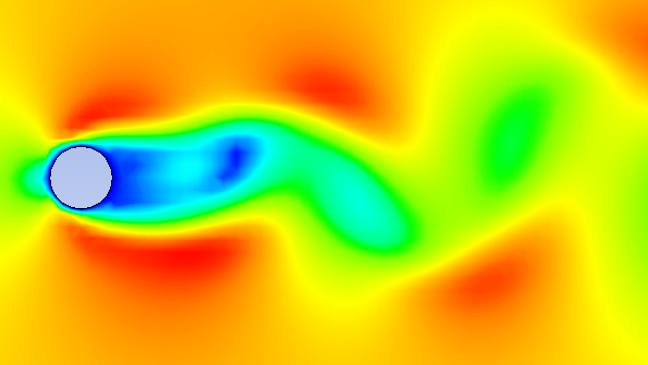
Time-Step Independence Is Not What You Think It Is: The Stiffness vs. CFL Trap

I was simulating vortex shedding behind a cylinder at Re = 100. My explicit compressible solver gave plausible results at Δt = 1e-5 seconds, but to be “safe,” I ran it at Δt = 1e-7. The simulation took four days to capture three shedding cycles. When I mentioned this to a postdoc, she asked: “Why not use a pressure-projection method? You’re resolving sound waves that don’t matter.”

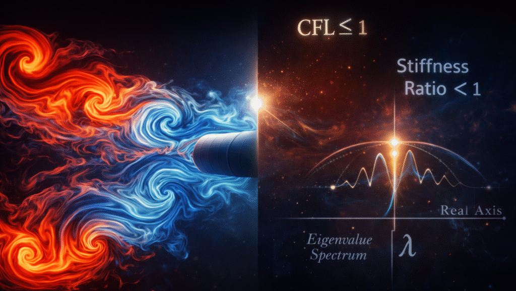
She was right. I was paying for stability against acoustic stiffness, not accuracy for vortex dynamics. This was my introduction to the crucial distinction between CFL-limited stability and numerical stiffness—two concepts often conflated, but demanding completely different solutions.

The Two Different Constraints:

Let’s diagnose a real problem—boundary layer flow with an anisotropic mesh. This isn’t exotic; it’s what happens when you resolve near-wall turbulence.

Case Study: The Anisotropic Grid Problem

Consider air at 20 m/s over a surface:

Streamwise spacing: Δx = 2×10^-4 m (resolving streamwise structures)
Wall-normal spacing: Δy_min = 2×10^-6 m (resolving viscous sublayer)
Kinematic viscosity: ν = 1.5×10^-5 m²/s
Speed of sound: c ≈ 340 m/s

Now compute the explicit stability limits:

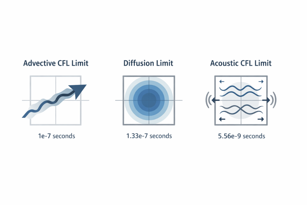
1. Advective CFL Limit:

$$
\begin{array}{rcl}
\Delta t_{\text{CFL}}
\le \frac{\min(\Delta x_{min}, \Delta y_{\min})}{u_{\max}}
= \frac{\min(2\times10^{-4},\, 2\times10^{-6})}{20}
= \frac{2\times10^{-6}}{20}
= 1\times10^{-7}\ \text{s}
\end{array}
$$

2. Diffusion Stability Limit:

$$
\begin{array}{rcl}
\Delta t_{\text{diff}}
&\le& 0.5 \, \frac{\Delta y_{\min}^{2}}{\nu} \
&=& 0.5 \, \frac{(2\times10^{-6})^{2}}{1.5\times10^{-5}} \
&=& 1.33\times10^{-7}\ \text{s}
\end{array}
$$

So far, advection and diffusion give similar limits (~1e-7 s). But here’s where it gets painful:

3. Acoustic CFL (for compressible solvers):

$$
\begin{array}{rcl}
\Delta t_{\text{acoustic}}
&\le& \frac{\min(\Delta x_{min}, \Delta y_{\min})}{u_{\max} + c} \
&=& \frac{2\times10^{-6}}{20 + 340} \
&=& 5.56\times10^{-9}\ \text{s}
\end{array}
$$

That’s 20× smaller. You’re taking 20 time steps to satisfy acoustics for every step the flow physics actually needs. The vortices shed at ~0.2 Hz (period = 5 s), so you’d need:

$\frac{5 s}{5.56×10^{-9} s/step} ≈ 900 million $

900 million steps per shedding cycle! That’s not computing—that’s insanity.

The Diagnostic That Changed My Workflow

Before you reduce Δt again, compute these ratios:

Diagnostic Python Pseudocode:

def diagnose_timestep_limits(grid, flow_params):
    dt_advective = CFL * min_cell_size / max_velocity
    dt_diffusive = 0.5 * min_cell_size**2 / max_diffusivity
    dt_acoustic = CFL * min_cell_size / (max_velocity + sound_speed)
    
    ratios = {
        'stiffness_suspicion': min(dt_diffusive, dt_acoustic) / dt_advective,
        'acoustic_dominance': dt_acoustic / dt_advective,
        'diffusion_dominance': dt_diffusive / dt_advective
    }
    
    if ratios['stiffness_suspicion'] < 0.1:
        print("Warning: Stiffness likely dictating Δt")
        if ratios['acoustic_dominance'] < 0.1:
            print("→ Acoustic stiffness. Consider incompressible formulation.")
        if ratios['diffusion_dominance'] < 0.1:
            print("→ Grid-induced stiffness. Consider implicit diffusion.")
    
    return ratios

For my boundary layer case:

dt_acoustic / dt_advective = 5.56e-9 / 1e-7 = 0.0556
Stiffness suspicion ratio: 0.0556 (definitely stiff)

The diagnostic screams: “Your Δt is limited by acoustics, not by the vortices you’re studying.”

What Researchers Actually Debate

The Methodological Split

For low-Mach vortex shedding (Mach ≈ 0.06 in my case), the literature shows three competing approaches:

Team Pressure-Projection (SIMPLE/PISO): “Filter acoustics entirely. Use elliptic pressure equation.”

Team All-Speed Compressible: “Use preconditioning to modify eigenvalues so pseudo-sound speed ≈ flow speed.” This approach is comprehensively detailed in [1] Turkel (1999) , which remains the standard reference for preconditioning techniques in CFD.

Team IMEX (Implicit-Explicit): “Treat stiff terms implicitly, non-stiff explicitly.” [2] Kennedy & Carpenter (2019) provide the modern framework for additive Runge-Kutta methods tailored to convection-diffusion-reaction systems.

All three produce valid results for standard benchmarks. The disagreement isn’t about correctness, but about computational efficiency and implementation complexity.

The Parallel Performance Reality Check

The real trade-off isn’t just “implicit vs explicit.” It’s about scalability on modern architectures.

Explicit methods have near-perfect weak scaling but suffer when stiffness forces tiny Δt. Implicit methods permit larger Δt but incur linear solver overhead. Let’s model this properly:

Let:

$N$ = number of cells
$\Delta t_e$ = explicit stability limit
$\Delta t_i$ = implicit allowable step (accuracy-limited)
$C_e$ = cost per cell per explicit step $\sim O(1)$
$C_i$ = cost per cell per implicit step $\sim O(\log N)$ (AMG complexity)
$E(P)$ = parallel efficiency on $P$ cores ($0 < E \leq 1$)

Total wall time:

$$
T_e = \frac{\Delta t_e}{T_{\text{sim}}} \cdot \frac{P \, E_e(P)}{N \, C_e}
$$

$$
T_i = \frac{\Delta t_i}{T_{\text{sim}}} \cdot \frac{P\,E_i(P)}{N\,C_i \log N}
$$

Implicit wins when:

$$
\frac{\Delta t_e}{\Delta t_i}
>
\frac{C_e}{C_i}
\cdot
\log N
\cdot
\frac{E_i(P)}{E_e(P)}
$$

For practical CFD:

$\frac{C_i}{C_e} \approx 50\text{–}100 \quad (\text{linear solver overhead})$
$\log N \approx 10\text{–}15 \quad \text{for } N = 10^{6}\text{–}10^{9}$
$\frac{E_e}{E_i} \approx 2\text{–}5 \quad (\text{explicit typically scales better})$

So implicit needs:

$$
\frac{\Delta t_e}{\Delta t_i} > 100 \cdot 15 \cdot 5 = 7500
$$

For the parameter ranges above, this estimate suggests implicit methods need roughly three orders of magnitude larger Δt to break even. For acoustic stiffness (ratio ≈ 20,000), implicit wins easily. For mild diffusion stiffness (ratio ≈ 10), explicit wins.

What I Still Struggle With

1. The Gray Area of Moderate Stiffness

When the stiffness ratio is 10–100 (not 20,000), the literature offers contradictory guidance:

Some papers show IMEX methods excelling
Others show stabilized explicit methods (RKC) winning on GPUs
[3] Pareschi & Russo (2005) provide rigorous analysis of IMEX schemes for hyperbolic systems with relaxation, but applying their stability conditions to complex 3D unstructured grids remains an open problem

My current heuristic: If I can afford the memory and my code already has a good linear solver, I go implicit. Otherwise, I test both and measure.

2. The Verification Gap

How do I know if my “stable” implicit simulation is correct? Explicit methods blow up obviously. Implicit methods can produce plausible-looking wrong answers through excessive numerical dissipation.

Consider: An implicit diffusion solver with too-large Δt doesn’t blow up—it just overdamps gradients. The vortices look “smoother.” Is that physical damping or numerical dissipation? Papers suggest monitoring solution time derivatives, but in practice, I’m never completely sure.

3. The Mesh Generation Feedback Loop

We’re taught: “Refine mesh until solution converges.” But refining Δy without considering Δt_diff = O(Δy²/ν) can make the problem stiff. Should we:

Accept stiffness and switch to implicit?
Keep mesh coarse where stiffness would occur?
Use anisotropic refinement with local time-stepping?

Most papers assume you’ve already chosen your method. Real CFD requires choosing method and mesh together, iteratively.

When Does Implicit Actually Win? A Quantitative Decision Framework

Let’s move beyond hand-waving. Here’s my current decision process:

Step 1: Diagnose before coding

Compute: dt_CFL, dt_diff, dt_acoustic
If min(dt_diff, dt_acoustic)/dt_CFL < 0.01:
    Problem is stiff → Choose method accordingly

Step 2: Select method based on stiffness source

if acoustic_dominated and Mach < 0.3:
    Use pressure-projection (incompressible) or preconditioning
elif diffusion_dominated and aspect_ratio > 50:
    Use IMEX with implicit diffusion (e.g., Kennedy & Carpenter)
elif both:
    Consider fully implicit
else:
    Explicit is fine

Step 3: Validate with cost model

Estimate: speedup_factor = Δt_implicit/Δt_explicit
Estimate: overhead_factor = (per_step_cost_ratio) × (scaling_penalty)
If speedup_factor > overhead_factor × 2:  # Conservative margin
    Implement implicit
Else:
    Keep explicit, consider algorithmic optimization

Step 4: Monitor, don’t assume

Log which cells limit Δt
Track stiffness indicators (rapid changes in solution time derivatives)
Be ready to switch methods if initial diagnosis was wrong

The Realization

Time-step independence isn’t about finding the smallest stable Δt. It’s about identifying which physical process dictates your Δt and deciding whether that process matters to your science.

For my vortex shedding, acoustics dictated Δt. But acoustics don’t matter for vortex dynamics. By switching to a pressure-projection method that filters acoustics, I gained a factor of 20,000 in Δt.

The mistake wasn’t using small Δt. The mistake was letting the wrong physics control my numerics.

Now, when a simulation acts unstable, I don’t reflexively reduce Δt. I ask:

What’s the smallest Δt that should work? (Based on CFL for the physics I care about)
What’s actually limiting Δt? (Acoustics? Diffusion? Something else?)
Do I care about that limiting physics? (If not, change discretization, not Δt)

Sometimes the answer is “reduce Δt.” Often, it’s “change your method.”

That distinction has saved me weeks of computation. More importantly, it’s changed how I think about CFD: not as “solving equations,” but as “selectively approximating physics to extract insight efficiently.”

References

I’m still learning. I still get this wrong sometimes. But now at least I know which mistakes are expensive, and which are just inelegant. The journey from CFD user to numerical analyst begins with understanding what’s actually limiting your time step, not just making it smaller until the warnings stop.

Questions for Discussion

Where’s the real threshold between “mild stiffness” and “switch to implicit”?
How do I verify that a large implicit time step isn’t quietly distorting the physics?
When do I change the discretization itself instead of just reducing Δt?

References

- Turkel, E. (1999). Preconditioning techniques in computational fluid dynamics. Annual Review of Fluid Mechanics, 31(1), 385-416.
- Kennedy, C. A., & Carpenter, M. H. (2019). Additive Runge-Kutta schemes for convection-diffusion-reaction equations. Applied Numerical Mathematics, 144, 35-57.
- Pareschi, L., & Russo, G. (2005). Implicit-Explicit Runge-Kutta schemes and applications to hyperbolic systems with relaxation. Journal of Scientific Computing, 25(1), 129-155.