Based on Liu et al. (2018), Dong et al. (2016), Zhan et al. (2020) · Computational Fluid Mechanics
The problem: vorticity is not the same as rotation
Ask any fluid dynamicist to point to a vortex in a flow field and they will likely reach for vorticity — the curl of the velocity vector, ∇ × V. It has an elegant mathematical definition, it is easy to compute, and it has been used as a proxy for rotation for well over a century. But there is a fundamental problem: vorticity does not distinguish between a fluid element that is genuinely spinning and one that is simply being sheared.
The clearest illustration comes from comparing two canonical 2D flows. In a Couette flow — a simple viscous flow between two parallel plates — the fluid near the wall has high vorticity purely because of the velocity gradient across the gap. No fluid particle is actually orbiting a common axis. In a 2D rigid rotation, by contrast, every particle traces a circle. Both flows can have identical vorticity magnitudes. Classical methods cannot tell them apart.
This ambiguity has real consequences. In the turbulent boundary layer, vorticity is large near the wall — not because there are strong vortices there, but because the mean shear is large. As Robinson noted, the association between regions of strong vorticity and actual vortices is remarkably weak in near-wall turbulence. The maximum vorticity does not even mark the centre of the vortex.
Key insight: Vorticity = rotation + shear. Classical vortex methods capture the sum. What researchers actually need is the rotation part alone — and for the first time, Rortex provides it.
Previous attempts: a generation of threshold-dependent workarounds
The limitations of raw vorticity prompted a generation of alternative criteria, all based on local analysis of the velocity gradient tensor ∇v. The tensor can be decomposed into a symmetric rate-of-strain part S and an antisymmetric rate-of-rotation part Ω. Four methods became standard:
| Method | Core idea | Key limitation |
|---|---|---|
| Δ criterion | Vortex = region where ∇v has complex eigenvalues (Δ > 0); streamlines spiral around a centre | Threshold sensitive; gives no axis direction or swirl strength |
| Q criterion | Vortex = region where Q = ½(‖Ω‖² − ‖S‖²) > 0; rotation dominates strain | Threshold is arbitrary: same DNS data can show breakdown or no breakdown |
| λ₂ (lambda-2) | Vortex = connected region where second eigenvalue of S² + Ω² is negative | Improper threshold produces “fake” vortex tube breakdowns |
| Swirling strength λci | Vortex = region with complex eigenvalue pair; λci quantifies swirl rate | Mixes shear and rotation; cannot isolate rigid-rotation axis in 3D |
The common thread: every method produces a scalar field, requires the user to pick a threshold, and provides no definitive answer about where a vortex begins and ends. Change the threshold and the vortex topology can change entirely.
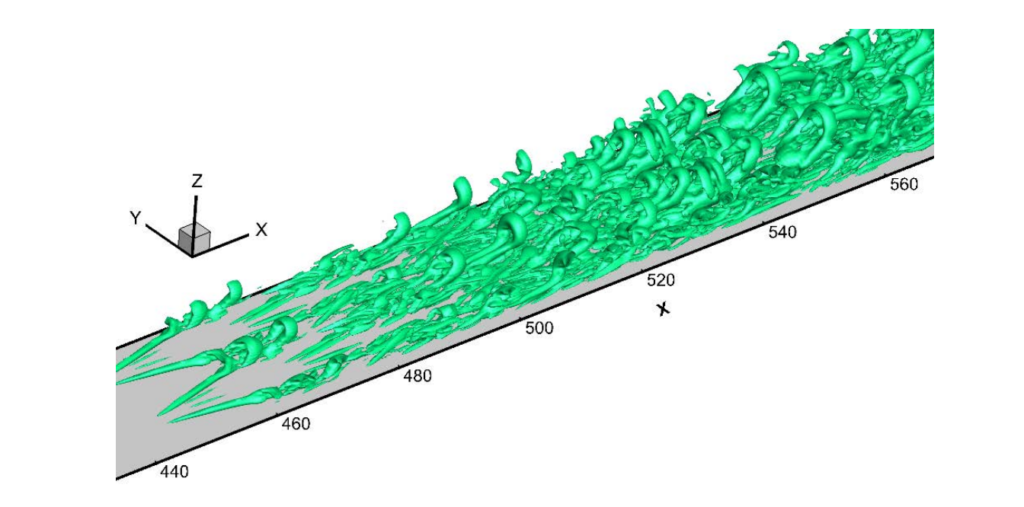
“Even if the same DNS data on late boundary layer transition is employed, vortex breakdown will be exposed for some large threshold in Q-criterion while no vortex breakdown can be found for some smaller threshold. This will directly influence one’s understanding of the mechanism of turbulence generation.”
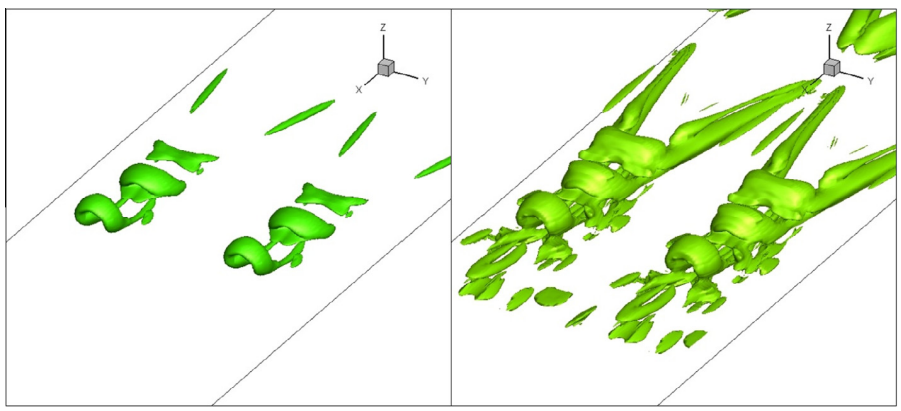
Source: Dong, Yan & Liu (2016), Applied Mathematical Modelling, 40, 500–509, Fig. 1.
Source: Dong, Yan & Liu (2016), Applied Mathematical Modelling, 40, 500–509, Fig. 1.or a threshold-independent, physically meaningful definition.
The solution: Rortex — isolating rigid rotation from the velocity gradient
Rortex, introduced by Liu, Gao, Tian and Dong in 2018, cuts the Gordian knot by directly isolating the rigid-body rotation component of local fluid motion. The approach proceeds in two stages: first find the axis of rotation, then measure only the rotation around it — discarding shear contributions entirely.
Stage 1 — finding the rotational axis
For a fluid element to rotate about a specific axis, the velocity gradient tensor, when expressed in a frame aligned with that axis, must satisfy two conditions: the velocity components along the axis must have zero derivatives in the two perpendicular directions. Formally, if the axis is Z, then ∂W/∂X = 0 and ∂W/∂Y = 0.
Liu et al. proved, using real Schur decomposition, that for any velocity gradient tensor a proper rotation matrix Q always exists such that the transformed tensor meets these conditions. The Z-direction of that rotated frame is the rotation axis r. When the tensor has only real eigenvalues — meaning no coherent swirling motion exists — the Rortex magnitude is automatically zero.
∇V = Q · ∇v · Q⁻¹ → finds axis r where ∂W/∂X = ∂W/∂Y = 0
Stage 2 — measuring rotation strength without shear
Once aligned with the rotational axis, the 2D cross-section of the velocity gradient in the X–Y plane is analysed. This 2×2 slice can be written in terms of two quantities: α, the amplitude of the oscillating (shear) component, and β = ½(∂V/∂X − ∂U/∂Y), which is the half-vorticity in the plane. Rigid rotation requires |β| > α. When this holds, the Rortex magnitude R is:
R = 2(|β| − α) when β² > α² (zero otherwise)
The full Rortex vector is then R = R·r — a magnitude that measures only genuine angular velocity, pointed along the true rotation axis. This decomposition is provably unique: there is no other way to separate the vorticity tensor into a pure-rotation part and a non-rotation part.
The vorticity decomposition it implies
One of the most significant theoretical consequences of Rortex is what it reveals about vorticity itself. The vorticity vector ∇ × V can be decomposed as:
∇ × V = R + S
where R is the Rortex vector (the purely rotational part) and S is a non-rotational shear vector. Vorticity can only serve as a proxy for rotation when S = 0 — that is, only in the limiting case of a perfectly rigid fluid. In all real turbulent flows, the shear component pollutes the vorticity signal.
Practical advantages: what Rortex reveals that other methods miss
Beyond mathematical elegance, Rortex offers four concrete practical advantages over existing methods, demonstrated in DNS and LES studies of turbulent boundary layers and jet-in-cross-flow configurations.
1. Rortex lines stay inside vortex tubes
In classical vortex analysis, vorticity lines are known to penetrate the surfaces of lambda-2 iso-surfaces — they can enter, cross, and exit what is being presented as a “vortex tube.” This is physically inconsistent: a true vortex tube should be impenetrable to the vortex lines that define it. Rortex lines, by contrast, always run parallel to the vortex surface and never leak through it. This follows directly from the construction of Rortex as the purely rotational component.
2. Vortex tubes can terminate inside the flow field
Classical Helmholtz theorems state that vorticity tubes cannot end in the interior of a fluid — they must either form closed loops or terminate at a boundary. Rortex tubes, however, can be generated, develop, and end entirely within the flow field. This means Rortex tubes are genuinely local objects, whereas vorticity tubes are globally constrained artefacts of the vorticity definition.
3. Eliminating spurious “zigzag” structures
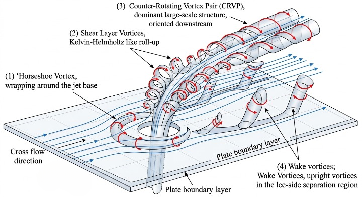
In LES of jet-in-cross-flow at different blowing ratios, Zhan et al. (2020) found that Q criterion, lambda-2, and swirling strength all produced a jagged, zigzag crown structure on the windward face of the jet hole — a feature inconsistent with the smooth 3D streamlines in that region. Rortex identified a smooth, clean vortex boundary. The zigzag features are artefacts of the shear contamination in those methods; Rortex, having separated rotation from shear, is simply not susceptible to this class of error.
4. Multiple representations beyond iso-surfaces
Because Rortex is a vector quantity rather than a scalar, it supports a richer vocabulary of visualisation: Rortex iso-surfaces, Rortex vector fields on those surfaces, Rortex lines as 3D curves, and Rortex tubes with varying strength along their length. This suite of tools gives researchers independent ways to verify that a detected structure is a genuine vortex and not an artefact.
Engineering application: tracking vortex shedding in a jet in cross flow
The jet-in-cross-flow (JICF) configuration is of direct engineering relevance in film cooling of turbine blades, where coolant jets protect metal surfaces from hot combustion gases. The effectiveness of this protection is strongly coupled to the vortex dynamics near the jet hole.
Zhan et al. (2020) used Rortex with LES and power spectrum density analysis across two blowing ratios (BR = 0.1 and BR = 0.5). The results showed that Rortex not only identifies vortex structures more accurately — it also enables quantitative spectral analysis by providing a physically meaningful scalar that can be monitored at fixed points in the flow.
| Blowing ratio | Dominant shedding mechanism | Frequency |
|---|---|---|
| BR = 0.1 | Horseshoe vortex sheds from leading edge of jet hole | ~60 Hz |
| BR = 0.1 | Shear vortex shedding | ~180 Hz |
| BR = 0.5 | Hovering vortex carried out of hole and shed (horseshoe shedding suppressed) | ~200 Hz |
The power spectrum density of the Rortex value at monitoring points clearly resolved these shedding frequencies. This kind of quantitative, spectral characterisation of vortex dynamics is difficult with scalar methods because those methods conflate rotation with shear, blurring the signal that would otherwise isolate periodic rotational events.
Why this matters beyond the numbers
The impact of Rortex reaches beyond better-looking flow visualisations. At its core, it resolves a conceptual ambiguity that has persisted since Helmholtz first defined vortex tubes in the mid-nineteenth century. Vorticity is a mathematical convenience, not a physical object. A fluid element with high vorticity may be rotating vigorously, or it may simply be sandwiched between layers moving at different speeds.
“Vorticity is not vortex vector: ∇ × V = R + S. Vorticity can be used to show the vortex structure properly only when S = 0 — where the fluid becomes rigid.”
Rortex provides a mathematically unique decomposition of the vorticity tensor into a pure rotation part and a non-rotational shear part. This uniqueness is not merely convenient — it means Rortex is not one method among many but the only correct answer to the question “how fast is this fluid element spinning, and around what axis?”
Computationally, the method is also practical. A single post-processing step on a regular laptop takes approximately one minute per time step for a 60-million-grid-point DNS dataset. The algorithm is based on the standard LAPACK DGEES subroutine for real Schur decomposition, making it straightforward to implement in any existing CFD post-processing pipeline.
Open questions and future directions
Despite its theoretical completeness, Rortex raises as many questions as it answers. The earlier λ₂ and vortex-filament hybrid method of Dong et al. (2016) demonstrated that even well-defined rotation cores are not necessarily vortex tubes: the Λ-vortices studied in that work were pairs of open rotation cores through which vorticity lines passed freely. Rortex’s own tubes can terminate in the flow interior. This challenges long-standing assumptions about vortex topology that remain embedded in turbulence models and engineering correlations.
There is also the question of Lagrangian consistency. The methods discussed here are all Eulerian — they give a snapshot of rotation at one instant. Objective, frame-independent Lagrangian methods offer a complementary perspective, particularly for slowly evolving coherent structures. How Rortex-based Eulerian identification relates to these Lagrangian structures remains an active area of research.
Finally, the decomposition ∇ × V = R + S opens a new avenue for turbulence modelling. If the energy cascade in turbulence is driven primarily by the rotational component R — as seems physically plausible — then models that operate on R rather than the full vorticity vector may offer improved accuracy. This hypothesis has yet to be rigorously tested across a wide range of flow configurations.
In summary: Rortex is not just an improved visualisation tool. It is a fundamental mathematical re-framing of what it means for a fluid to rotate — one with implications for how we model, analyse, and ultimately control turbulence.
Primary sources: Liu C., Gao Y., Tian S., Dong X. (2018). “Rortex — A new vortex vector definition and vorticity tensor and vector decompositions.” Physics of Fluids, 30(3), 035103. · Dong Y., Yan Y., Liu C. (2016). “New visualization method for vortex structure in turbulence by lambda2 and vortex filaments.” Applied Mathematical Modelling, 40, 500–509. · Zhan J., Chen Z., Li C., Hu W., Li Y. (2020). “Vortex identification and evolution of a jet in cross flow based on Rortex.” Engineering Applications of Computational Fluid Mechanics, 14(1), 1237–1250.