There’s a quiet revolution happening at the intersection of machine learning and turbulence modelling, and it doesn’t look like what most people expect. It isn’t a neural network replacing your CFD solver. It isn’t a deep learning surrogate that takes a mesh and spits out a pressure field. It’s something more interesting, and in some ways more unsettling: an algorithm that reads your high-fidelity flow data and writes you a mathematical equation.
That equation, if the method works, is a correction to your RANS closure. One you can actually read. One whose terms correspond to something physical. One that a fluid mechanician can look at and say — yes, that makes sense, and here is why.
This is symbolic regression applied to turbulence modelling, and in the last two years it has moved from a niche idea to one of the most actively pursued directions in the field.
The problem symbolic regression is solving
To appreciate why this matters, it helps to recall why data-driven turbulence modelling exists at all.
RANS models — the k-ε, the k-ω SST, the Spalart-Allmaras — are engineering workhorses. They’re fast, robust, and embedded into every industrial solver from Fluent to OpenFOAM. But they carry a fundamental deficiency: the Reynolds stress closure is built on the Boussinesq hypothesis, which assumes the Reynolds stress tensor is linearly proportional to the mean strain rate. That assumption holds reasonably well in attached, equilibrium boundary layers. It fails — sometimes spectacularly — for separated flows, flows with strong streamline curvature, impinging jets, and anything involving significant stress anisotropy.
High-fidelity data from DNS and LES tells us exactly how the baseline RANS stress prediction is wrong, pointwise, in a given flow. The discrepancy field is computable. The question is what to do with it.
The first wave of data-driven approaches used neural networks to learn a mapping from local flow features (invariants of the strain and rotation rate tensors, turbulence quantities) to Reynolds stress corrections. Work by Wang, Wu and Xiao (2016–2018) established the physics-informed machine learning (PIML) framework that is now widely cited. Ling, Kurzawski and Templeton (2016) went further, embedding Galilean invariance directly into the architecture via a tensor-basis neural network, ensuring the learned closure respected the symmetries of the Navier-Stokes equations.
These methods work. Tested a posteriori, the corrected RANS solver outperforms the baseline on separated flows by meaningful margins. But they have two problems that have stubbornly refused to go away.
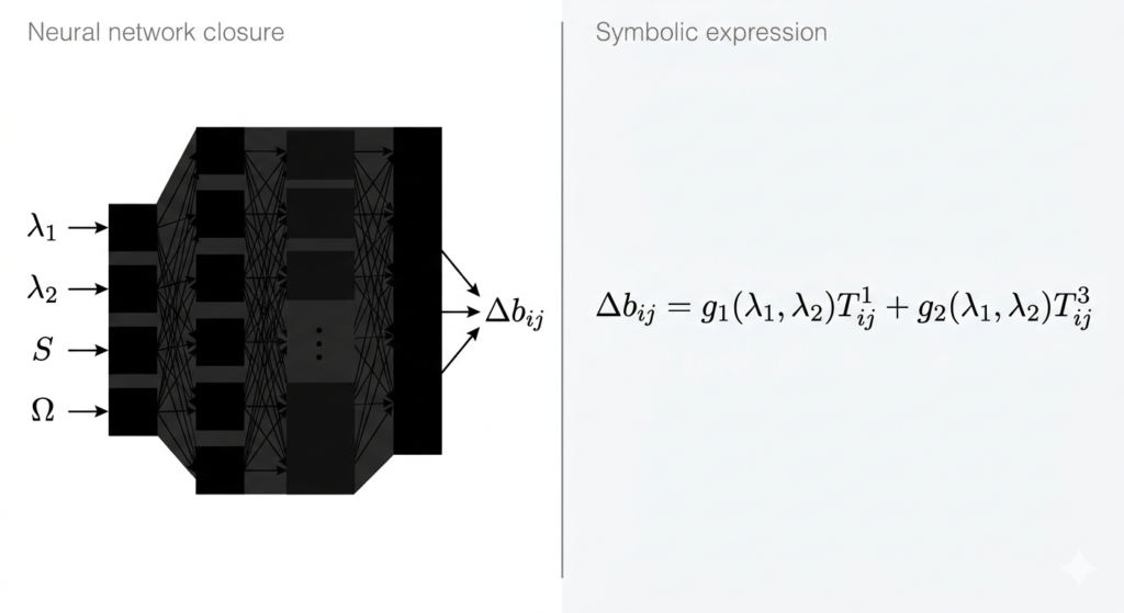
Interpretability. A neural network with hidden layers produces a closure you cannot read. You cannot extract physics from it. You cannot know whether it learned something about turbulence or something about the specific geometry it was trained on. You cannot hand it to a colleague and explain what it does. This is not merely an aesthetic complaint — it is an epistemological one. A model you cannot interpret is a model you cannot improve.
Generalisability. Neural network closures trained on periodic hills tend to fail on backward-facing steps. Trained on channel flow, they often degrade on flows with adverse pressure gradients. The learned mapping encodes dataset-specific behaviours alongside genuine physics, and the two are tangled in the weights of the network.
Symbolic regression is a direct attack on both problems.
What symbolic regression actually does
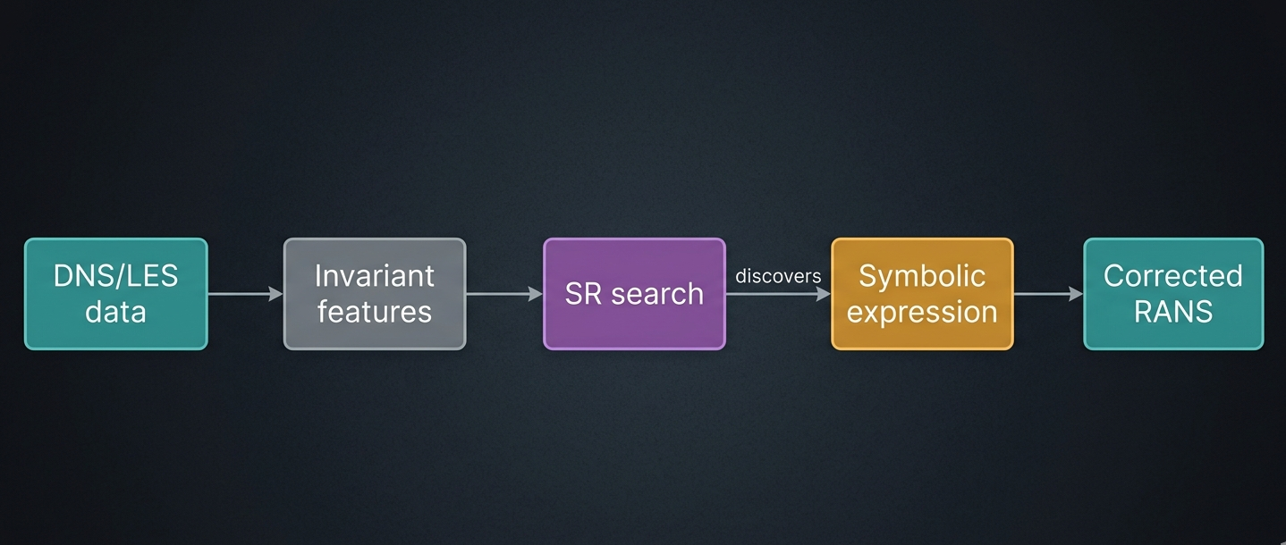
Symbolic regression (SR) is a form of machine learning that searches the space of mathematical expressions — rather than the space of real-valued parameters — to find a formula that best describes some data. Unlike linear regression (which finds coefficients for a fixed functional form) or neural networks (which fit parameters in a fixed architecture), SR discovers the functional form itself.
The search space is enormous. An expression can combine addition, multiplication, exponentiation, trigonometric functions, and any set of input features in arbitrarily nested combinations. Early SR methods used genetic programming to evolve expression trees. More recent approaches use deep learning — specifically recurrent neural networks or transformer-based sequence models — to generate candidate expressions, scored by a combination of accuracy and complexity, in a directed search that is orders of magnitude more efficient than random evolution.
The output is a compact algebraic expression. Something like:
\[\Delta b_{ij} = g_1(\lambda_1, \lambda_2) T^{(1)}_{ij} + g_2(\lambda_1, \lambda_2) T^{(3)}_{ij}\]
where \(b_{ij} = \tau_{ij}/2k – \delta_{ij}/3\) is the Reynolds stress anisotropy tensor, \(T^{(n)}_{ij}\) are tensor basis functions constructed from the mean strain and rotation rate tensors, \(\lambda_n\) are their scalar invariants, and \(g_n\) are scalar coefficients discovered by the algorithm from data.
This is not a black box. Every term is readable. Every coefficient has units you can check. Every tensor basis function has a physical interpretation in terms of strain and rotation.
The key results of the last two years
SpaRTA and the sparsity approach. Among the earliest systematic SR methods for turbulence was SpaRTA (Sparse Regression of Turbulent Stress Anisotropy), which frames the problem as sparse regression over a library of candidate tensor polynomials. Given DNS data for separated flows over periodic hills, a converging-diverging channel, and a curved backward-facing step, SpaRTA discovers compact additive corrections to the Reynolds stress constitutive equation. Critically, these corrections — verified in a posteriori CFD — improve predictions not just on the training geometry but on genuinely unseen cases including higher Reynolds numbers.
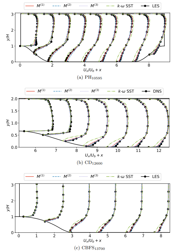
Figure 8 from Schmelzer et al. (2020): Streamwise velocity profiles for three separated flow geometries. SR-discovered models M⁽¹⁾–M⁽³⁾ (dashed) consistently recover the high-fidelity reference (DNS/LES, dots) where the baseline k-ω SST (solid) fails. Source: arXiv:1905.07510, reproduced with attribution.
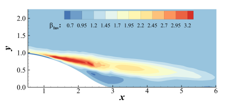
The Wu and Zhang SST-SR framework. Wu and Zhang (2023) applied SR to the SST model via field inversion. First, field inversion solves the inverse problem: given DNS data for the target flow, what scalar correction field \(\beta(\mathbf{x})\) multiplying the turbulence production term would make the SST predictions match the data? The field inversion problem is well-posed (given sufficient regularisation) and produces a pointwise correction field. SR then learns an algebraic expression mapping local flow invariants to \(\beta\). The result is a closed-form correction that can be embedded directly in the SST transport equations with zero additional computational cost. Tested on separated flows including the curved backward-facing step and periodic hills, the method demonstrates both accuracy improvement and generalisability to flows outside the training set.
Figure 5 from Wu & Zhang (2023): The optimised β correction field over the curved backward-facing step geometry. β > 1 (red) indicates regions where the SST production term is systematically underpredicted — concentrated in the recirculation core. SR then learns an algebraic expression that maps local flow invariants to this field. Source: arXiv:2304.11347, reproduced with attribution.
The Journal of Fluid Mechanics generalisation paper (2025). Perhaps the most physically interesting recent contribution is a JFM paper that frames the generalisation problem directly. The authors observe that data-driven closures fail to generalise because they conflate universal flow physics with dataset-specific behaviours. Their solution is architectural: they decompose SR-discovered corrections into inner-layer, outer-layer, and pressure-gradient components, and demonstrate that only the inner-layer component is truly generalisable. Retaining only this component, combined with selective outer-layer corrections for specific flow classes, yields symbolic corrections that are compact, physically motivated, and generalise to unseen aerofoil geometries and Reynolds numbers outside the training set. The resulting models outperform both Spalart-Allmaras and SST in a priori and a posteriori tests.
The Physics of Fluids coupled DA-SR framework (July 2025). A paper just published in Physics of Fluids by Liao, Sun, Liu and Zhang introduces a mutually coupled framework for data assimilation and symbolic regression. A key limitation of prior FIML-SR approaches was that they applied SR to steady-state solutions, and the discovered model, when coupled back into the RANS solver, could introduce numerical instability. The coupled framework iterates between data assimilation (which provides the training signal) and SR (which produces the algebraic expression) until mutual consistency is achieved. Applied to high Reynolds number flows past aerofoils at large angles of attack — one of the most challenging cases for RANS due to massive separation — the method produces a model with improved accuracy, robust stability, and demonstrated generalisability across aerofoil families. This is a meaningful step because stability during solver coupling has historically been the weakest link in the FIML-SR pipeline.
Why interpretability is not just a nicety
One way to think about the black-box versus white-box distinction is to ask: what can you learn from the model once you have it?
A neural network closure tells you, essentially, nothing. You can measure its accuracy. You can probe its sensitivity to inputs by computing gradients. But the knowledge it contains is locked in millions of floating-point numbers that don’t correspond to physical concepts.
A symbolic expression is different. When SpaRTA discovers that the dominant correction to the Reynolds stress in a separated flow scales with a particular invariant of the rotation rate tensor, that is a finding about turbulence physics. When Wu and Zhang find that the SST production correction is a function of the ratio of turbulent timescale to mean strain timescale, that is interpretable: it says the model needs to know whether the turbulence is in structural equilibrium with the mean flow or lagging behind it. These insights can inform the next generation of hand-crafted models — the kind that get built into commercial solvers and used for the next twenty years.
This is the deeper promise of symbolic regression for turbulence. It’s not just a better black box. It’s a method for doing physics.
The open problems
None of this is solved. Several challenges remain that are worth being honest about.
The a priori to a posteriori gap. SR is almost always trained on DNS data by minimising the discrepancy between the learned expression and the true Reynolds stress field, evaluated at fixed mean flow conditions (the frozen-RANS assumption). But when the discovered model is actually coupled back into the solver, the mean flow changes, and the model is evaluated at conditions it was never trained on. This a posteriori degradation is a generic problem for all data-driven closures, and SR is not immune. The coupled DA-SR framework addresses this partially, but a general solution remains elusive.
Extrapolation to higher Reynolds numbers. DNS data is expensive. Essentially all training cases are at moderate Reynolds numbers \(Re \leq 10^5\). Whether discovered symbolic models extrapolate to the \(Re \sim 10^7\) regimes relevant for aerospace applications is an open question. The JFM generalisation paper gives some encouraging evidence, but the Reynolds number gap remains large.
Multi-physics flows. Almost all SR turbulence work has focused on incompressible, isothermal, single-phase flows. Compressibility, heat transfer, and multiphase dynamics introduce additional unclosed terms beyond the Reynolds stress. Extending SR to these regimes is technically possible but has not yet been done systematically.
The search space explosion. The space of possible symbolic expressions grows superexponentially with expression depth. Current methods manage this with complexity penalties and physics-based constraints (unit consistency, Galilean invariance), but the search is still expensive and not always reliable. Methods that leverage large language models — AutoTurb being a recent example — are beginning to use the world knowledge embedded in LLMs to bias the search toward physically plausible expressions. It is early, but the direction is interesting.
A note on where this connects to the broader RANS problem
It’s worth stepping back and placing symbolic regression in the context of the field as a whole.
The fundamental difficulty with RANS is not that the models are badly parameterised — it’s that the Boussinesq hypothesis is wrong for a wide class of practically relevant flows. Any correction that remains within the Boussinesq framework, however sophisticated, is correcting a structurally deficient model. The Reynolds stress anisotropy — the deviation of the stress tensor from isotropy, quantifiable through tools like the Lumley triangle or the barycentric map — is precisely the quantity that the Boussinesq hypothesis suppresses by construction.
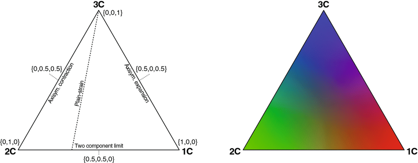
Symbolic regression, in its most ambitious form, targets the full Reynolds stress anisotropy tensor directly, without assuming a linear eddy viscosity. This is what tensor-basis SR is doing: it searches for explicit algebraic expressions for the full \(b_{ij}\) tensor in terms of mean flow invariants, respecting the physical symmetries and realizability constraints that any valid Reynolds stress model must satisfy. In this sense, the most sophisticated SR approaches are discovering explicit algebraic stress models — a class of closures that the turbulence modelling community has been trying to derive analytically for decades.
The difference is that SR discovers them from data rather than from closure assumptions. Whether the discovered expressions are more physically faithful, and whether they generalise better than their hand-crafted analogues, is an empirical question that the field is actively answering.
Where I think this is going
My own view is that the interpretable, symbolic approach is the right direction, and that the current moment — where the tooling is mature enough to produce useful results but the physics being extracted is still early — is an unusually productive time to be working in this space.
The specific combination of field inversion (to extract correction targets from high-fidelity data), tensor-basis decomposition (to enforce physical invariances), and symbolic regression (to produce algebraic, human-readable expressions) is now a reasonably well-established pipeline. The frontier is in making it robust — in a posteriori stability, in high Reynolds number extrapolation, in coupling with data assimilation, and in extending to more complex flow physics.
There’s also a meta-question lurking here that I find genuinely interesting: is there a compact algebraic model that correctly describes the Reynolds stress anisotropy for a broad class of flows, waiting to be discovered? The success of SR on specific flow families suggests the answer might be yes, at least locally. Finding out is worth the effort.
If you’re working on data-driven turbulence modelling, or have thoughts on the interpretability-accuracy tradeoff, I’d like to hear from you. The comment section is open.
References available on request.
Further Reading
Structural Limits of Linear Eddy-Viscosity Models in the Planar Jet