Okay, real talk for a minute. Last month, I almost submitted a paper with results that were mathematically beautiful and physically impossible. My pressure-based solver said everything was perfect—residuals at \(10^{-6}\), drag coefficient stable to four decimals. Then my advisor asked the simple question: “How much mass is actually entering versus leaving the domain?”
Turns out, 0.95% of the mass had just… disappeared. The solver never mentioned it. No error messages. No warning flags. Just silent conservation violation. This is the dirty secret of pressure-based solvers that nobody teaches you in CFD 101.
The SIMPLE Algorithm’s Little White Lie
Here’s what they don’t tell you in class: the SIMPLE algorithm (Semi-Implicit Method for Pressure-Linked Equations) that powers 80% of industrial CFD simulations, can exhibit non-negligible global mass imbalance unless additional correction and monitoring strategies are employed.
When you solve:
\(\nabla^2 p’ = \nabla \cdot \mathbf{u}^*\)
You’re actually solving an approximation. The full correction equation should be:
\( a_P \mathbf{u}P’=\sum a_{nb}\mathbf{u}_{nb}’-V_P\nabla p’ \)
But SIMPLE says: “Eh, let’s ignore those neighbor terms \(\sum a_{nb} \mathbf{u}_{nb}’\). They’re probably small.” SIMPLE linearizes the pressure–velocity coupling by neglecting certain velocity correction dependencies in the pressure equation, which are only partially recovered through iteration.
Spoiler: They’re not always small. Especially near boundaries, corners, or anywhere the flow is doing something interesting.
How I Caught My Solver Red-Handed
Let me walk you through exactly what happened in my simulation (a simple pipe flow, because even “simple” cases fail).
The Setup:
- Software: ANSYS Fluent (but this applies to OpenFOAM, Star-CCM+, everyone)
- Case: Turbulent pipe flow at Re=10,000
- Solver: Pressure-based, SIMPLE, second-order everything
- Convergence: Residuals below \(10^{-6}\), monitor points stable
The Check My Professor Made Me Do:
- Mass flow in: \(\dot{m}_{in} = 0.523 \text{ kg/s}\)
- Mass flow out: \(\dot{m}_{out} = 0.518 \text{ kg/s}\)
- Error: \(\epsilon = 0.956\%\)
That’s 1% of my mass just… gone. Not lost to numerics, not a discretization error—this is the algorithm literally not conserving mass between iterations.
Why Your Residuals Are Lying to You
Here’s the kicker: The continuity residual you monitor?
\(R_{cont} = \sum_{cells} |\nabla \cdot (\rho \mathbf{u})| V_{cell}\)
This can be tiny while mass imbalance is huge. Why? Because positive and negative errors cancel out in the sum. A cell gaining mass and a cell losing mass look fine together.
Actual Diagnostic You Should Run (Python/Pseudo-Code):
python
def check_mass_conservation(simulation):
    mass_in = sum(boundary_mass_flux('inlet'))
    mass_out = sum(boundary_mass_flux('outlet'))
    mass_walls = sum(boundary_mass_flux('wall'))  # Should be zero!

    imbalance = abs(mass_in - mass_out - mass_walls)
    relative_error = imbalance / (0.5*(abs(mass_in) + abs(mass_out)))

    return relative_error  # If > 0.1%, you have problems
Real-World Consequences (From My Lab’s Failures)
Case 1: The Pump That Shouldn’t Work
A friend in turbomachinery spent weeks optimizing an impeller. SIMPLE said: “Great! 5% efficiency improvement!” Prototype built, tested… actually 2% worse. Why? The pressure correction was artificially reducing recirculation zones in the simulation. Mass wasn’t being properly redistributed in the blade passages.
Case 2: The “Efficient” Heat Exchanger
Our lab designed a compact heat exchanger. Simulation showed perfect temperature distribution. Manufacturing showed hot spots. The issue? The solver was “leaking” mass at manifold junctions, changing the flow distribution between channels.
Case 3: My Almost-Published Paper
I was simulating particle-laden flow. The VOF (Volume of Fluid) method coupled with SIMPLE was losing 0.2% of droplet mass per time step. Over 1000 time steps? 20% mass error. And the residuals? Beautiful. Convergence? Perfect.
The Rhie-Chow Ghost in the Machine
If you’re using collocated grids (and you probably are), you’re using Rhie-Chow interpolation. It’s what prevents the “checkerboard” pressure pattern. But here’s its dirty secret:
\(\mathbf{u}_f = \bar{\mathbf{u}}_f+(\frac{V}{a})_f\underbrace{[\nabla p_f- \frac{p_N – p_P}{d{P_N}}]}\)
That term in braces? It’s artificial. It’s not physics. It’s numerical stabilization that can create or destroy mass flux at faces.
In regions of high pressure curvature (near stagnation points, corners, shock waves), this term becomes significant. And your mass conservation? Gone.
When SIMPLE Becomes Too Simple
The algorithm variants matter:
| Algorithm | Mass Conservation | When It Lies |
|---|---|---|
| SIMPLE | Poor | Always, but especially with large Δt |
| SIMPLEC | Better | Still fails with skewed grids |
| PISO | Good for transients | Can lag density in compressible flows |
| PIMPLE | Best overall | But 2-3x more expensive |
Here’s my rule of thumb after burning myself three times:
- SIMPLE: Only for quick, rough estimates
- SIMPLEC: Daily workhorse, but check mass balance
- PISO/PIMPLE: Anything serious, anything transient
The Compressibility Trap
“Pressure-based solvers are fine below Mach 0.3” – every textbook ever.
Reality check: The issue isn’t Mach number, it’s pressure-density coupling stiffness:
\(S = \left(\frac{\partial \rho}{\partial p}\right)_T \cdot \frac{\Delta p}{\rho_0}\)
A slight heads-up, \(S\) is a heuristic indicator, not a formal stability criterion.
If \(S > 0.001\), your pressure-based solver starts losing mass conservation. For air at room temperature:
\(\frac{\partial \rho}{\partial p} = \frac{1}{RT} \approx 3.5 \times 10^{-5} \text{ Pa}^{-1}\)
A pressure drop of just 1000 Pa gives \(S = 0.035\)—way into the danger zone. And guess what? Most internal flows have pressure drops in the 1000-10,000 Pa range.
What Actually Works (From Trial and Error)
1. The Coupled Solver Solution
Switching from segregated (SIMPLE) to coupled solver fixes most issues. Yes, it uses 2-3x more memory. Yes, it might be slower per iteration. But it actually conserves mass.
ANSYS Fluent: Use “Coupled” instead of “SIMPLE”
OpenFOAM: Use “pimpleFoam” instead of “simpleFoam”
Star-CCM+: Use “Segregated Flow” with “Coupled” energy
Repeating the same case with a coupled solver reduced mass imbalance below 0.02% under identical discretization.
2. The Tight Tolerance Band-Aid
If you must use SIMPLE:
- Pressure correction tolerance: \(10^{-8}\) (not \(10^{-6}\))
- Under-relaxation: 0.3 for pressure (not 0.7)
- Do at least 2-3 extra iterations after “convergence”
3. The Monitoring You MUST Implement
python
# Pseudo-monitoring for every simulation
monitoring_points = {
    'mass_imbalance': 'calculate every iteration',
    'global_mass': 'should be constant for closed domains',
    'species_conservation': 'for passive scalars',
    'energy_balance': 'if solving energy'
}

thresholds = {
    'mass_error': 'alarm if > 0.1%',
    'drift_rate': 'alarm if > 0.01%/iteration'
}
The Student’s Survival Guide
Here’s what I wish someone had told me when I started:
Quick Checks Before You Trust Results:
- Calculate mass balance – not residuals
- Monitor a passive scalar – if it drifts, mass is leaking
- Check closed domains – mass should be constant
- Compare with coupled solver – if different, SIMPLE is lying
When to Panic:
- Error < 0.01%: You’re fine
- 0.01% < Error < 0.1%: Suspicious, investigate
- 0.1% < Error < 1%: Problematic, fix before continuing
- Error > 1%: Your results are physically meaningless
Script I Actually Use:
python
# Quick mass balance check (conceptual)
def sanity_check(simulation):
    issues = []

    # Mass conservation
    m_in = get_mass_flow('inlet')
    m_out = get_mass_flow('outlet')
    if abs(m_in - m_out)/m_in > 0.001:
        issues.append(f"Mass imbalance: {(m_in-m_out)/m_in*100:.2f}%")

    # Species conservation (if applicable)
    for species in simulation.species:
        total = integrate(species.concentration)
        if total.drift_rate() > 0.001:
            issues.append(f"Species {species.name} drifting")

    return issues
The Bottom Line
In finite-precision, under-relaxed, segregated implementations, pressure-based solvers can exhibit persistent mass imbalance that is not reflected in residual norms. The question isn’t “if” but “how much” and “does it matter for my case.”
For quick conceptual designs? SIMPLE is fine.
For anything going into a paper, a prototype, or production? Use coupled solvers or at least PIMPLE.
And for the love of all that is holy: check your mass balance. Not your residuals. Your actual, physical mass entering and leaving the domain.
Because nothing is more embarrassing than building something that shouldn’t work according to your own simulation… and then having to explain why the real world doesn’t match your beautiful, mass-leaking, mathematically elegant CFD results.
This discussion applies primarily to steady or pseudo-steady segregated pressure-based solvers on collocated grids, under typical industrial under-relaxation settings.
🔥 Controlled Burn: If your CFD software doesn’t make it easy to check mass conservation, it’s not engineering software—it’s a video game with fancy graphics.
💡 Pro Tip for Students: Put mass balance checks in your simulation template. Make it run automatically every 100 iterations. You’ll thank yourself later.
📚 Further Reading (Actual Useful Stuff):
- Navigating CFD Flow Solvers: Segregated vs. Coupled Methods & Their Applications
- OpenFOAM’s PIMPLE algorithm documentation
- Understanding Fluent Solvers: Pressure-based vs Density-based
Made this mistake? Share your horror story below. Let’s commiserate over bad CFD results together.
Ans also don’t forget to explore the Playground page for some mini quizzes and videos!


